Chapter 3 Geographic analysis

Under construction…

3.1 Clean coordinates

Some occurrence records may have invalid coordinates (e.g., not in decimal format, not between -180 and 180 [lon] or -90 and 90 [lat], not within the bounds of the country listed) or coordinates with suspicious validity (e.g., zero/zero coordinates, lat and long are equal, coordinates match the country centroid), and these issues must be dealt with before conducting geographical analyses. coord_clean can be used to remove bad coordinates using a variety of validity tests (see function details). Additionally, the number of digits can be specified for automatic rounding of coordinates.

Example code for cleaning coordinates:

library(fungarium)

#import sample data set
data(agaricales_updated) #United States Agaricales records

#see Table 2.1 for preview of agaricales data set

Table 3.1: Preview of agaricales data set
	id	institutionCode	scientificName	scientificNameAuthorship	recordedBy	year	eventDate	occurrenceRemarks	habitat	country	stateProvince	county	decimalLatitude	decimalLongitude	references
269864	9961160	O	Galerina mniophila	(Lasch) Kühner	Gro Gulden	1997	1997-11-15		young Douglas fir forest	United States	Oregon	Benton			https://mycoportal.org/portal/collections/individual/index.php?occid=9961160
313673	454144	MICH	Mycena galopus	(Pers.) P. Kumm.	A. H. Smith	1935	1935-11-30			USA	California	Humboldt	41.0595	-124.1419	https://mycoportal.org/portal/collections/individual/index.php?occid=454144
157092	4570238	iNaturalist	Armillaria mellea	(Vahl) P. Kumm.	Cindy Trubovitz	2017	2017-01-07	<p>Growing from the base of an old log</p>; <a href=‘https://www.inaturalist.org/observations/5244247’ target=’_blank’ style=‘color: blue;’> Original observation #5244247 (iNaturalist)</a>		United States	California		32.80975	-117.1295	https://mycoportal.org/portal/collections/individual/index.php?occid=4570238
281279	456630	MICH	Hygrophorus olivaceoalbus	(Fr.) Fr.	R. L. Shaffer	1956	1956-09-16			USA	Idaho	Valley	44.8753	-115.9017	https://mycoportal.org/portal/collections/individual/index.php?occid=456630
32558	2270252	MICH	Cortinarius	(Pers.) Gray	S. J. Mazzer	1970	1970-05-31	[Collection is stored in Cortinarius indeterminate box]		USA	Michigan	Cheboygan			https://mycoportal.org/portal/collections/individual/index.php?occid=2270252
522392	345316	MICH	Crepidotus malachius var. phragmocystidiosus	Hesler & A.H. Sm.	A. H. Smith	1959	1959-08-18	Notes with collection North Amer. Sp. Crepidotus 1965 pg. 58.	On hardwood	USA	Michigan	Chippewa			https://mycoportal.org/portal/collections/individual/index.php?occid=345316
234305	526338	OSC	Cortinarius montanus	Kauffman	Jim Trappe	1976	1976-09-08	Old-growth Tsme	Old-growth Tsme	USA	Oregon	Lane			https://mycoportal.org/portal/collections/individual/index.php?occid=526338
356189	2287069	DUKE	Schizophyllum commune	Fr.	D. Porter	1998	1998-04-00			United States	Georgia	Clarke	33.95	-83.383333	https://mycoportal.org/portal/collections/individual/index.php?occid=2287069
237907	2357852	WTU	Cortinarius rubicundulus	(Rea) A. Pearson	L. L. Norvell, SAR.	1992	1992-11-17		Rotten wood/ duff. Sequoia, Tan Oak.	U.S.A.	California	Mendocino			https://mycoportal.org/portal/collections/individual/index.php?occid=2357852
140361	6920708	iNaturalist	Amanita pachycolea	D.E. Stuntz	Taylor Bates	2017	2017-11-13	<a href=‘https://www.inaturalist.org/observations/8797347’ target=’_blank’ style=‘color: blue;’> Original observation #8797347 (iNaturalist)</a>		United States	Oregon		44.665631	-123.242596	https://mycoportal.org/portal/collections/individual/index.php?occid=6920708

#clean coordinates
agaricales_cleaned <- coord_clean(agaricales_updated)

## 'non-numeric coord' test: 11788 records removed.

## 'non-valid coord' test: 0 records removed.

## 'zero' test: 0 records removed.

## 'equal' test: 0 records removed.

## Running 'countries' test...

## 'countries' test: 392 records removed.

## Running 'centroids' test...

## 'centroids' test: 0 records removed.

## Total records removed: 12180

3.2 Assigning records to geographic grid cells

Before plotting geographic trait data within bounding “boxes,” record coordinates are used to assign each record to individual grid cells. hex_grid can be used to create a world map grid of hexagonal cells with a specific area (in square kilometers). See the code below for a demonstration on how to assign occurrence records to individual grid cells.

Example code for finding trait records and calculating enrichment factors:

#make hex grid
grid <- hex_grid(20000)

#convert lat/long points to sf geometry
agaricales_sf <- sf::st_as_sf(agaricales_cleaned,
                              coords = c("decimalLongitude", "decimalLatitude"),
                              crs = "+proj=latlong +ellps=WGS84 +datum=WGS84")

#convert to cylindrical equal area projection coordinates
agaricales_sf <- sf::st_transform(agaricales_sf,
                                  crs = "+proj=cea +ellps=WGS84 +datum=WGS84")

#assign points to grid cells
agaricales_grid <- sf::st_join(grid, agaricales_sf, join=sf::st_contains, left=FALSE)

3.3 Calculate trait enrichment per grid cell

After assigning records to specific grid cells, trait enrichment can be calculated for each cell using the enrichment function. See code below for an example on calculating fire-associated enrichment.

Example code for calculating enrichment factors:

#find fire-associated records
string1 <- "(?i)charred|burn(t|ed)|scorched|fire.?(killed|damaged|scarred)|killed.by.fire"
string2 <- "(?i)un.?burn(t|ed)"
trait_rec <- find_trait(agaricales_grid, pos_string=string1, neg_string=string2)

#find fire-associated enrichment per grid cell
fire_enrich <- enrichment(agaricales_grid, trait_rec, ext_var="geometry", by="hex")

#filter out hex cells with low amount of occurrences
fire_enrich <- fire_enrich[fire_enrich$freq>=5,]

3.4 Visualize trait enrichment

Once enrichment values have been calculated, annotated grid cells can be plotted on a world map using trait_map. Additionally, world map can be cropped to a specific region, if desired.

Example code for making trait map:

#plot trait data on world map
library(ggplot2)
fire_enrich <- sf::st_as_sf(fire_enrich) #convert enrichment table back to sf
map <- trait_map(fire_enrich, aes_mapping = aes(fill=trait_ratio),
                 color=NA, alpha=0.95, size=0.1)
map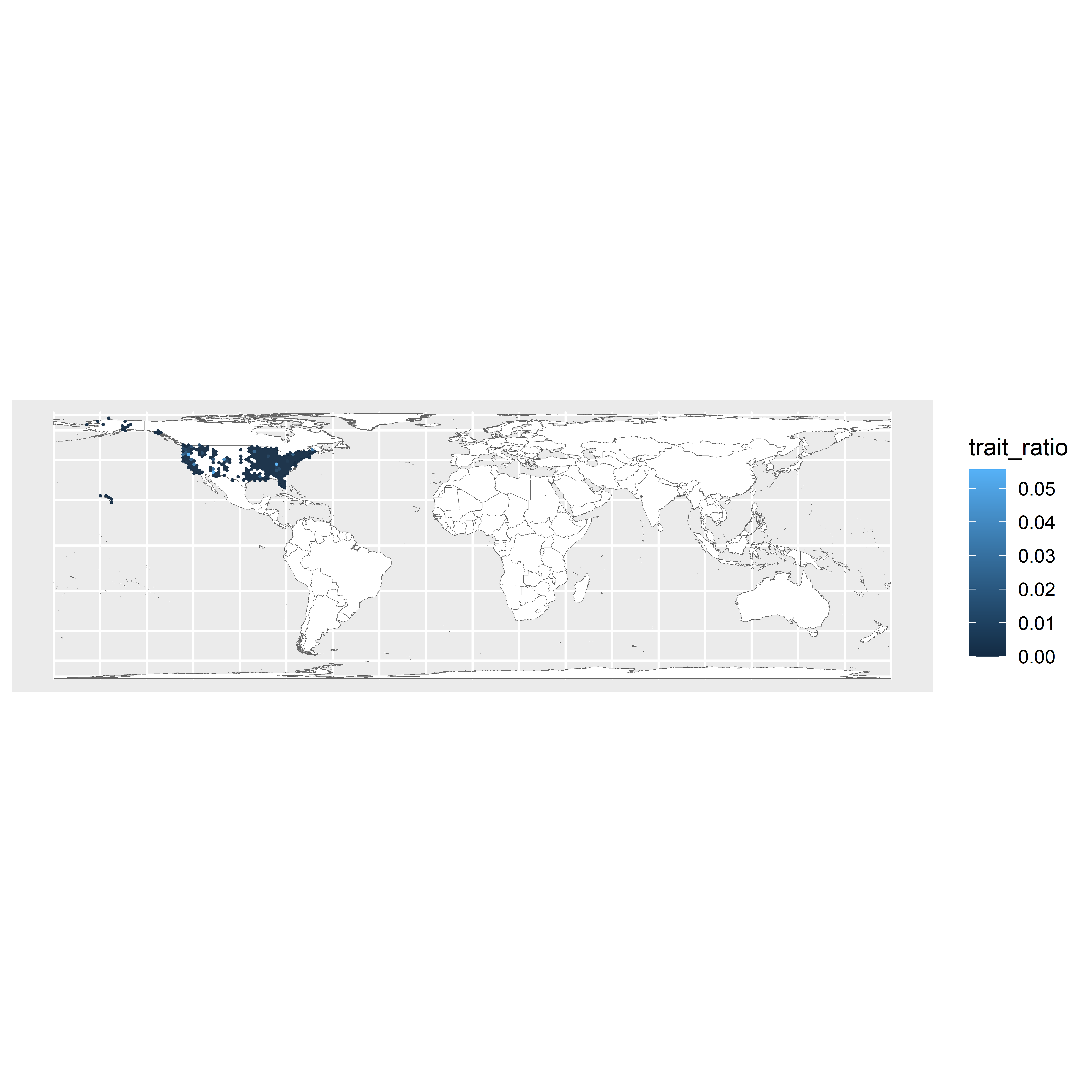

Figure 3.1: World map showing fire-associated enrichment via 20,000km2 grid cells

Example code for making trait map of specific region:

#Because sample data in from US only, crop world map to focus on US region 
map+
  ylim(c(300000,6000000))+
  xlim(c(-18000000,-6000000))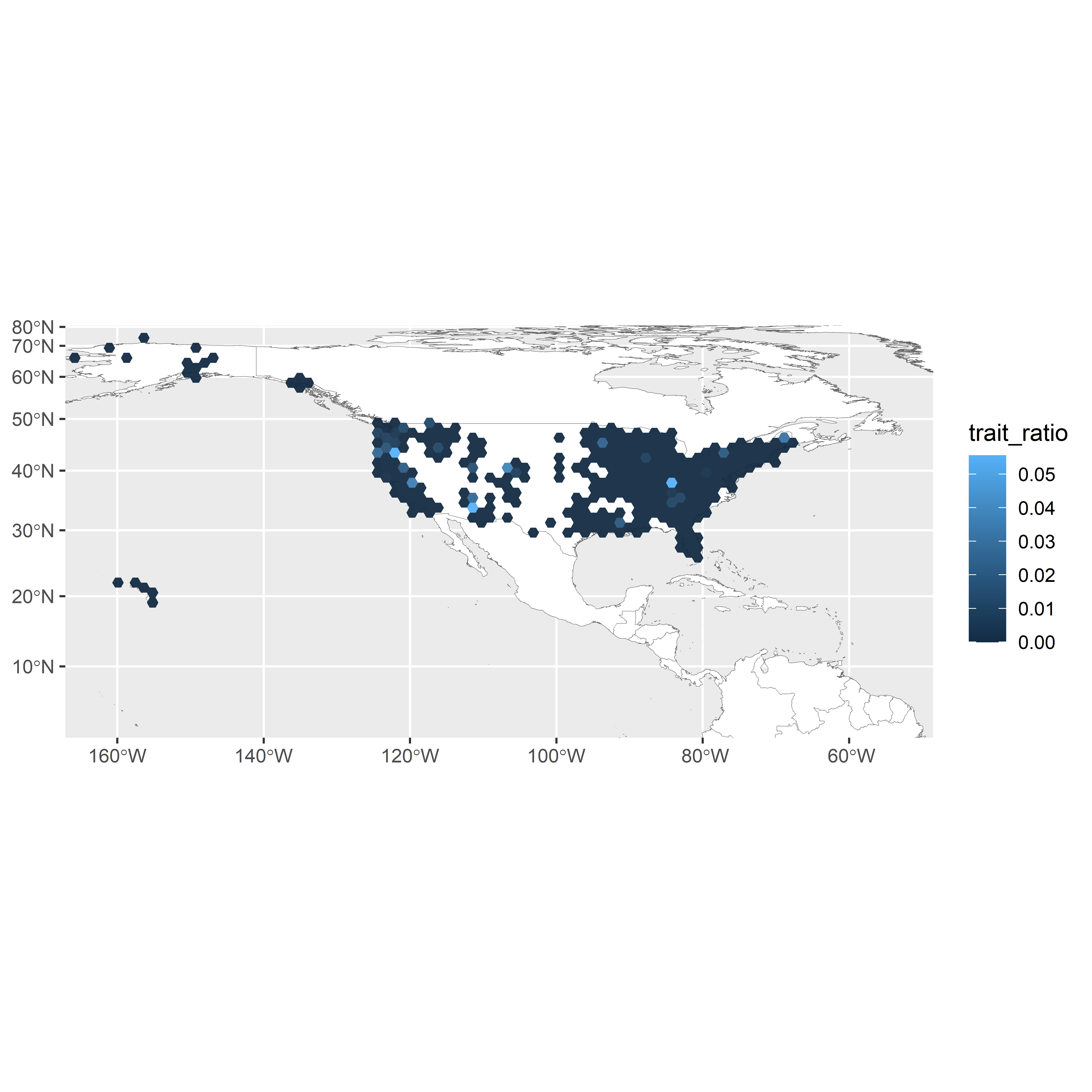

Figure 3.2: United States map showing fire-associated enrichment via 20,000km2 grid cells